
What is a Mathematical Model ???
Representation of reality by means of abstractions. The models focus on important parts of a system (at least, that she is interested in a specific model type), downplaying others.Models are created using modeling tools.
Types of Modeling:

* Mental model: first perception of the problem at
mental. It is the first play of ideas that are generated intuitively
on the problem at hand.
mental. It is the first play of ideas that are generated intuitively
on the problem at hand.
* Verbal Model: it is the first attempt to formalize language
characteristics of the problem. In this model performsfirst formal approach to the problem.
* Graphic model: the set of images and graphics support
to help locate the functional relations that prevail in
system to be studied.
* Physical Model: consists of an assembly that can operate
as a real testbed.They are usually
laboratory-scale simplifications that allow
more detailed observations. Not always easy to build.
as a real testbed.They are usually
laboratory-scale simplifications that allow
more detailed observations. Not always easy to build.
* Mathematical Model: seeks to formalize in mathematical languagerelations and variations you want to represent and analyze.
Normally expressed as differential equations and
this reason may also be known as differential model.
* Analytical Model: arises when the differential model has
solution. This is not always possible, especially when
differential models are formulated on differential
Partial.
solution. This is not always possible, especially when
differential models are formulated on differential
Partial.
* Numerical Model: arises when using numerical techniques
to solve differential models. They are very common when
differential model has no analytical solution.
to solve differential models. They are very common when
differential model has no analytical solution.
* Computational Model: refers to a program
computer that allows analytical or numerical models
can be solved more quickly. They are very useful for
implement numerical models because these are based on
iterative process can be long and tedious.
computer that allows analytical or numerical models
can be solved more quickly. They are very useful for
implement numerical models because these are based on
iterative process can be long and tedious.
Components of a Mathematical Model
Dependent Variables
Independent Variables
Parameters
Functions of Force
Operators
Round-off
Round-off errors arise because it is impossible to represent all real numbers exactly on a finite-state machine (which is what all practical digital computers are).
All non-zero digits are considered significant. For example, 91 has two significant figures (9 and 1), while 123.45 has five significant figures (1, 2, 3, 4 and 5).
CASE A: In rounding off numbers, the last figure kept should beunchanged if the first figure dropped is less than 5. | For example, if only one decimal is to be kept, then 6.422 becomes 6.4. |
CASE B: In rounding off numbers, the last figure kept should beincreased by 1 if the first figure dropped is greater than 5. | For example, if only two decimals are to be kept, then 6.4872 becomes 6.49. Similarly, 6.997 becomes 7.00. |
CASE C: In rounding off numbers, if the first figure dropped is 5, and all the figures following the five are zero or if there are no figures after the 5, then the last figure kept should be unchanged if that last figure is even. | For example, if only one decimal is to be kept, then 6.6500 becomes 6.6. For example, if only two decimals are to be kept, then 7.485 becomes 7.48. |
CASE D: In rounding off numbers, if the first figure dropped is 5, and all the figures following the five are zero or if there are no figures after the 5, then the last figure kept should be increased by 1 if that last figure is odd. | For example, if only two decimals are to be kept, then 6.755000 becomes 6.76. For example, if only two decimals are to be kept, 8.995 becomes 9.00. |
CASE E: In rounding off numbers, if the first figure dropped is 5, and there are any figures following the five that are notzero, then the last figure kept should be increased by 1. | For example, if only one decimal is to be kept, then 6.6501 becomes 6.7. For example, if only two decimals are to be kept, then 7.4852007 becomes 7.49. |
Truncation and discretization error
Truncations errors are committed when an iterative method is terminated or a mathematical procedure is approximated, and the approximate solution differs from the exact solution. Similarly, discretization induces a discretization errorbecause the solution of the discrete problem does not coincide with the solution of the continuous problem. For instance, in the iteration in the sidebar to compute the solution of3x3 + 4 = 28, after 10 or so iterations, we conclude that the root is roughly 1.99 (for example). We therefore have a truncation error of 0.01.
Once an error is generated, it will generally propagate through the calculation. For instance, we have already noted that the operation + on a calculator (or a computer) is inexact. It follows that a calculation of the type a+b+c+d+e is even more inexact.
What does it mean when we say that the truncation error is created when we approximate a mathematical procedure. We know that to integrate a function exactly requires one to find the sum of infinite trapezoids. But numerically one can find the sum of only finite trapezoids, and hence the approximation of the mathematical procedure. Similarly, to differentiate a function, the differential element approaches to zero but numerically we can only choose a finite value of the differential element.
Example :
Using the graphical method, find the solution of the systems of equations

Since f(0.5) = 0.125 the root is in [0, 0.5].
Since f(0.25) = -0.73 the root is in [0.25, 0.5].
Since f(0.375) = -0.38 the root is in [0.375, 0.5].
Since f(0.4375) = -0.15 the root is in [0.4375, 0.5].
Since f(0.46875) = -0.018 the root is in [0.46875, 0.5].
Since f(0.484375) = 0.05 the root is in [0.46875, 0.484375].
... and so we approach the root 0.472834 It is superfluous to say that it is easy to computerize this method. Then we have the root in less than a second.
• You are guaranteed the convergence of the root lock.
• Easy implementation.
• management has a very clear error.
Disadvantages
• The convergence can be long.
• No account of the extreme values (dimensions) as


The algorithm is first in the class of Householder's methods, succeeded by Halley's method.
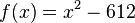
For example, if one wishes to find the square root of 612, this is equivalent to finding the solution to
Secant method


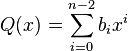
A polynomial function is a function that can be defined by evaluating a polynomial. A function ƒ of one argument is called a polynomial function if it satisfies
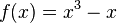
For example, the function ƒ, taking real numbers to real numbers, defined by
Müller's method is based on the secant method, which constructs at every iteration a line through two points on the graph of f. Instead, Müller's method uses three points, constructs the parabola through these three points, and takes the intersection of the x-axis with the parabola to be the next approximation.
The three initial values needed are denoted as xk, xk-1 and xk-2. The parabola going through the three points (xk, f(xk)), (xk-1, f(xk-1)) and (xk-2, f(xk-2)), when written in the Newton form, is
Note that xk+1 can be complex, even if the previous iterates were all real. This is in contrast with other root-finding algorithms like the secant method or Newton's method, whose iterates will remain real if one starts with real numbers. Having complex iterates can be an advantage (if one is looking for complex roots) or a disadvantage (if it is known that all roots are real), depending on the problem.

Bairstow's Method
Bairstow's approach is to use Newton's method to adjust the coefficients u and v in the quadratic x2 + ux + v until its roots are also roots of the polynomial being solved. The roots of the quadratic may then be determined, and the polynomial may be divided by the quadratic to eliminate those roots. This process is then iterated until the polynomial becomes quadratic or linear, and all the roots have been determined.
Long division of the polynomial to be solved
 and a remainder cx + d such that
 and remainder gx + h with
 , and the
  are functions of u and v. They can be found recursively as follows.
After eight iterations the method produced a quadratic factor that contains the roots -1/3 and -3 within the represented precision. The step length from the fourth iteration on demonstrates the superlinear speed of convergence.
 ,
,  , and
, and  , polynomial long division gives a solution of the equation
is less than that of .
If we take as the divisor, giving the degree of as 0, i.e.
  :
:
 we obtain:
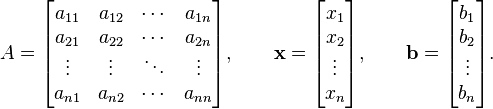
In mathematics, a matrix (plural matrices, or less commonly matrixes) is a rectangular array of numbers, such as
 Kinds of Matrixs


A = 

Root-Finding Equations
There are three kinds of methods to solve equations:
Graphics Methods
Open methods
Methods Closed
Graphics Methods
Systems of equations or simultaneous equations can also be solved by the graphical method.
To do that, we draw the graph for each of the equation and look for a point of intersection between the two graphs. The coordinates of the point of intersection would be the solution to the system of equations.
If the two graphs do not intersect - which means that they are parallel - then there is no solution.
Using the graphical method, find the solution of the systems of equations
y + x = 3
y = 4x - 2
Solution :
Draw the two lines graphically and determine the point of intersection from the graph. 
Features:
• Calculations are not accurate. • They have limited practical value.
• Allows initial estimate values.
• Allows understanding of the properties of
functions.
• They can help prevent failures in the methods.
• in general can be considered closed as ¨ closed¨

• Calculations are not accurate. • They have limited practical value.
• Allows initial estimate values.
• Allows understanding of the properties of
functions.
• They can help prevent failures in the methods.
• in general can be considered closed as ¨ closed¨
Closed Methods
They are limiting the search domain. Most
known are:
• Bisection Method
• False Position Method
known are:
• Bisection Method
• False Position Method
Bisection Method
Also known as method:
• Binary Court.
• Partition.
• Bolzano.
It is a type of incremental search is based on dividing the always in the middle interval and the change of sign on
interval.
• Binary Court.
• Partition.
• Bolzano.
It is a type of incremental search is based on dividing the always in the middle interval and the change of sign on
interval.

Example:
The equationt3 + 4 t2 - 1 = 0has a positive root r in [0,1]. f(0)<0 and f(1)>0.
Since f(0.5) = 0.125 the root is in [0, 0.5].
Since f(0.25) = -0.73 the root is in [0.25, 0.5].
Since f(0.375) = -0.38 the root is in [0.375, 0.5].
Since f(0.4375) = -0.15 the root is in [0.4375, 0.5].
Since f(0.46875) = -0.018 the root is in [0.46875, 0.5].
Since f(0.484375) = 0.05 the root is in [0.46875, 0.484375].
... and so we approach the root 0.472834 It is superfluous to say that it is easy to computerize this method. Then we have the root in less than a second.
Advantages
• You are guaranteed the convergence of the root lock.
• Easy implementation.
• management has a very clear error.
Disadvantages
• The convergence can be long.
• No account of the extreme values (dimensions) as
possible roots.
False Position Method

In numerical analysis, the false position method or regula falsi method is a root-finding algorithm that combines features from the bisection method and the secant method.
Like the bisection method, the false position method starts with two points a0 and b0 such that f(a0) and f(b0) are of opposite signs, which implies by the intermediate value theorem that the function f has a root in the interval [a0, b0]. The method proceeds by producing a sequence of shrinking intervals [ak, bk] that all contain a root of f.
At iteration number k, the number

is computed. As explained below, ck is the root of the secant line through (ak, f(ak)) and (bk, f(bk)). If f(ak) and f(ck) have the same sign, then we set ak+1 = ck and bk+1 =bk, otherwise we set ak+1 = ak and bk+1 = ck. This process is repeated until the root is approximated sufficiently well.
The above formula is also used in the secant method, but the secant method always retains the last two computed points, while the false position method retains two points which certainly bracket a root. On the other hand, the only difference between the false position method and the bisection method is that the latter uses ck = (ak + bk) /
Example code
#include#include double f(double x) { return cos(x) - x*x*x; } double FalsiMethod(double s, double t, double e, int m) { int n,side=0; double r,fr,fs = f(s),ft = f(t); for (n = 1; n <= m; n++) { r = (fs*t - ft*s) / (fs - ft); if (fabs(t-s) < e*fabs(t+s)) break; fr = f(r); if (fr * ft > 0) { t = r; ft = fr; if (side==-1) fs /= 2; side = -1; } else if (fs * fr > 0) { s = r; fs = fr; if (side==+1) ft /= 2; side = +1; } else break; } return r; } int main(void) { printf("%0.15f\n", FalsiMethod(0, 1, 5E-15, 100)); return 0; }
Open Methods Newton's Raphson Method
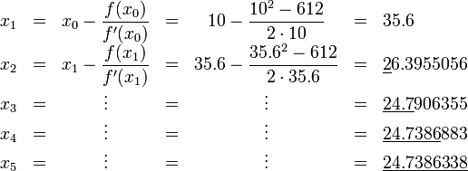
In numerical analysis, Newton's method(also known as the Newton–Raphson method), named after Isaac Newton and Joseph Raphson, is perhaps the best known method for finding successively better approximations to the zeroes (or roots) of a real-valued function. Newton's method can often converge remarkably quickly, especially if the iteration begins "sufficiently near" the desired root. Just how near "sufficiently near" needs to be, and just how quickly "remarkably quickly" can be, depends on the problem. This is discussed in detail below. Unfortunately, when iteration begins far from the desired root, Newton's method can easily lead an unwary user astray with little warning. Thus, good implementations of the method embed it in a routine that also detects and perhaps overcomes possible convergence failures. Given a function ƒ(x) and its derivative ƒ '(x), we begin with a first guess x0. Provided the function is reasonably well-behaved a better approximation x1 is

The process is repeated until a sufficiently accurate value is reached:

An important and somewhat surprising application is Newton–Raphson division, which can be used to quickly find the reciprocal of a number using only multiplication and subtraction.
The algorithm is first in the class of Householder's methods, succeeded by Halley's method.
Example
Square root of a number
Consider the problem of finding the square root of a number. There are many methods of computing square roots, and Newton's method is one.For example, if one wishes to find the square root of 612, this is equivalent to finding the solution to


Secant method
In numerical analysis, the secant method is a root-finding algorithm that uses a succession of roots of secant lines to better approximate a root of a function f. The secant method can be thought of as a finite difference approximation of Newton's method. However, the method was developed independent of Newton's method, and predated the latter by over 3000 years. 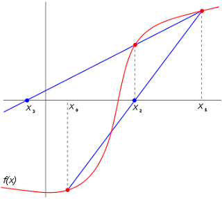
The secant method is defined by the recurrence relation

As can be seen from the recurrence relation, the secant method requires two initial values, x0 and x1, which should ideally be chosen to lie close to the root.
Example
#include#include double f(double x) { return cos(x) - x*x*x; } double SecantMethod(double xn_1, double xn, double e, int m) { int n; double d; for (n = 1; n <= m; n++) { d = (xn - xn_1) / (f(xn) - f(xn_1)) * f(xn); if (fabs(d) < e) return xn; xn_1 = xn; xn = xn - d; } return xn; } int main(void) { printf("%0.15f\n", SecantMethod(0, 1, 5E-11, 100)); return 0;
form f(x) = cos(x) − x3 = 0
After running this code, the final answer is approximately 0.865474033101614. The initial, intermediate, and final approximations are listed below, correct digits are underlined.


Fixed Point Method
If we can say
and we supose
X--->f(x)=0
X--->x+g(x)=0
then
X=g(x)

Fixed point iteration for a general function g(x) for the four cases of interest. Generalizations of the two cases of positive slope shown are shown on the left, and illustrate monotonic convergence and divergence. The cases where g(x) has negative slope are shown on the right, and illustrate oscillating convergence and divergence. The top pair of panels illustrate strong and weak attractors, while the bottom pair of panels illustrate strong and weak repellers.

Polynomial Roots
In mathematics, a polynomial is an expression of finite length constructed from variables (also known as indeterminates) and constants, using only the operations of addition, subtraction, multiplication, and non-negative, whole-number exponents. For example, x2 − 4x + 7 is a polynomial, but x2 − 4/x + 7x3/2 is not, because its second term involves division by the variable x and because its third term contains an exponent that is not a whole number.

For example, the function ƒ, taking real numbers to real numbers, defined by

Müller's Method
Müller's method is a root-finding algorithm, a numerical method for solving equations of the form f(x) = 0. It is first presented by D. E. Müller in 1956.Müller's method is based on the secant method, which constructs at every iteration a line through two points on the graph of f. Instead, Müller's method uses three points, constructs the parabola through these three points, and takes the intersection of the x-axis with the parabola to be the next approximation.
The three initial values needed are denoted as xk, xk-1 and xk-2. The parabola going through the three points (xk, f(xk)), (xk-1, f(xk-1)) and (xk-2, f(xk-2)), when written in the Newton form, is
![y = f(x_k) + (x-x_k) f[x_k, x_{k-1}] +
(x-x_k) (x-x_{k-1}) f[x_k, x_{k-1}, x_{k-2}], \,](http://upload.wikimedia.org/math/0/7/d/07d074d029f2eff141bd8463a5280472.png)
![y = f(x_k) + w(x-x_k) + f[x_k, x_{k-1},
x_{k-2}] \, (x-x_k)^2 \,](http://upload.wikimedia.org/math/0/e/f/0efe4e93a0231e0fab93005e94e52b75.png)
![w = f[x_k,x_{k-1}] + f[x_k,x_{k-2}] -
f[x_{k-1},x_{k-2}]. \,](http://upload.wikimedia.org/math/5/b/e/5be82acd77afa985a33a7beb2cfd6d8b.png)
![x_{k+1} = x_k - \frac{2f(x_k)}{w \pm
\sqrt{w^2 - 4f(x_k)f[x_k, x_{k-1}, x_{k-2}]}}.](http://upload.wikimedia.org/math/f/4/2/f4295e4a61122746e796cccc5653415f.png)
Note that xk+1 can be complex, even if the previous iterates were all real. This is in contrast with other root-finding algorithms like the secant method or Newton's method, whose iterates will remain real if one starts with real numbers. Having complex iterates can be an advantage (if one is looking for complex roots) or a disadvantage (if it is known that all roots are real), depending on the problem.

Bairstow's Method
Bairstow's approach is to use Newton's method to adjust the coefficients u and v in the quadratic x2 + ux + v until its roots are also roots of the polynomial being solved. The roots of the quadratic may then be determined, and the polynomial may be divided by the quadratic to eliminate those roots. This process is then iterated until the polynomial becomes quadratic or linear, and all the roots have been determined.
Long division of the polynomial to be solved
 and a remainder cx + d such that
 and remainder gx + h with
 , and the are functions of u and v. They can be found recursively as follows.
![\begin{bmatrix}u\\ v\end{bmatrix}
:=
\begin{bmatrix}u\\ v\end{bmatrix}
- \begin{bmatrix}
\frac{\partial c}{\partial u}&\frac{\partial c}{\partial
v}\\[3pt]
\frac{\partial d}{\partial u} &\frac{\partial d}{\partial v}
\end{bmatrix}^{-1}
\begin{bmatrix}c\\ d\end{bmatrix}
:=
\begin{bmatrix}u\\ v\end{bmatrix}
- \frac{1}{vg^2+h(h-ug)}
\begin{bmatrix}
-h & g\\[3pt]
-gv & gu-h
\end{bmatrix}
\begin{bmatrix}c\\ d\end{bmatrix}](http://upload.wikimedia.org/math/0/6/b/06bed931e9c9f2a198dc0b053f5fd43b.png)
Example
The task is to determine a pair of roots of the polynomial

| Nr | u | v | step length | roots |
|---|---|---|---|---|
| 0 | 1.833333333333 | -5.500000000000 | 5.579008780071 | -0.916666666667±2.517990821623 |
| 1 | 2.979026068546 | -0.039896784438 | 2.048558558641 | -1.489513034273±1.502845921479 |
| 2 | 3.635306053091 | 1.900693009946 | 1.799922838287 | -1.817653026545±1.184554563945 |
| 3 | 3.064938039761 | 0.193530875538 | 1.256481376254 | -1.532469019881±1.467968126819 |
| 4 | 3.461834191232 | 1.385679731101 | 0.428931413521 | -1.730917095616±1.269013105052 |
| 5 | 3.326244386565 | 0.978742927192 | 0.022431883898 | -1.663122193282±1.336874153612 |
| 6 | 3.333340909351 | 1.000022701147 | 0.000023931927 | -1.666670454676±1.333329555414 |
| 7 | 3.333333333340 | 1.000000000020 | 0.000000000021 | -1.666666666670±1.333333333330 |
| 8 | 3.333333333333 | 1.000000000000 | 0.000000000000 | -1.666666666667±1.333333333333 |
Synthetic Division
The polynomial remainder theorem follows from the definition of polynomial long division; denoting the divisor, quotient and remainder by, respectively, , , and , polynomial long division gives a solution of the equation is less than that of .
If we take
as the divisor, giving the degree of as 0, i.e. : we obtain:
Matrixs
In mathematics, a matrix (plural matrices, or less commonly matrixes) is a rectangular array of numbers, such as

- Column Matrix.or Column Vector. A matrix with only vertical entries is called a column matrix, whose order is denoted by (m x 1). It is a special case matrix with only one column.
- Row Matrix or Row Vector. A matrix with only horizontal entries is called a row matrix, denoted by (1 x n). It is a matrix with only one row and n columns.
- Furthermore, a matrix with only 1 entry (scalar) would be both a column and a row matrix.
- Square Matrix. A square matrix occurs when m=n or the number of rows equals the number of columns. An example of a (3 x 3) matrix is:
- Identity Matrix or Unit Matrix.. This square matrix is of order (n x n). The princpal (main) diagonal has all 1’s and the remaining elements are all 0’s.
- Diagonal Matrix. Like the identity matrix all entries not on the main diagonal are zero. Those entries on the main diagonal are not restricted to 1.
- Inverse of a Matrix. Given two square matrices A and B. If A B = B A = I then A is said to be invertible and B is the inverse of A.

- Symmetric Matrix. A square matrix is considered symmetric if and only if it is equal to its transpose.
- The following is an example of a (3 x 3) symmetric matrix:
- Skew-Symmetric Matrix. A square matrix is skew-symmetric if its negative is equal to its transpose.
- The following is an example of a skew-symmetric matrix:
- The diagonal terms of a skew-symmetric matrix must be zero.
- Triangular Matrix. Only square matrices can be considered upper or lower triangular. A matrix is upper triangular if all its coefficients below the main diagonal are all zero. Likewise, a matrix is lower triangular if all its coefficients above the main diagonal are all zero. This property can be used to find the determinant of a matrix. An example of the upper triangular matrix is:
- Zero or Null Matrix. The zero matrix occurs when all elements of a matrix are equal to zero. (Note: A zero matrix can be of various orders and thus not all operations can be done on them.)
Addition The sum A+B of two m-by-n matrices A and B is calculated entrywise:
- (A + B)i,j = Ai,j + Bi,j, where 1 ≤ i ≤ m and 1 ≤ j ≤ n.
- Scalar Multiplication
- The scalar multiplication cA of a matrix A and a number c (also called a scalar in the parlance of abstract algebra) is given by multiplying every entry of A by c:
- (cA)i,j = c · Ai,j.
- Transpose
- The transpose of an m-by-n matrix A is the n-by-m matrix AT (also denoted Atr or tA) formed by turning rows into columns and vice versa:
- (AT)i,j = Aj,i.
Matrix multiplication
Multiplication of two matrices is defined only if the number of columns of the left matrix is the same as the number of rows of the right matrix. If A is an m-by-n matrix and B is an n-by-p matrix, then their matrix product AB is the m-by-p matrix whose entries are given by dot-product of the corresponding row of A and the corresponding column of B:
- System Of Equations


A system of equations is a collection of two or more equations with a same set of unknowns. In solving a system of equations, we try to find values for each of the unknowns that will satisfy every equation in the system.
The equations in the system can be linear or non-linear. This tutorial reviews systems of linear equations.
The problem can be expressed in narrative form or the problem can be expressed in algebraic form.
Example of a narrative statement of a system of the equations:
The air-mail rate for letters to Europe is 45 cents per half-ounce and to Africa as 65 cents per half-ounce. If Shirley paid $18.55 to send 35 half-ounce letters abroad, how many did she send to Africa?
Example of an algebraic statement of the same system of the equations:

A system of linear equations can be solved four different ways:
Gaussian Elimination
In linear algebra, Gaussian elimination algorithm for solving systems of linear equations, finding the rank of a matrix, and calculating the inverse of an invertible square matrix. Gaussian elimination is named after German mathematician and scientist Carl Friedrich Gauss. is an
Elementary row operations are used to reduce a matrix to row echelon form. Gauss–Jordan elimination, an extension of this algorithm, reduces the matrix further to reduced row echelon form. Gaussian elimination alone is sufficient for many applications.
The process of Gaussian elimination has two parts. The first part (Forward Elimination) reduces a given system to either triangular or echelon form, or results in a degenerate equation with no solution, indicating the system has no solution. This is accomplished through the use of elementary row operations. The second step uses back substitution to find the solution of the system above.
Stated equivalently for matrices, the first part reduces a matrix to row echelon form using elementary row operations while the second reduces it to reduced row echelon form, or row canonical form.
Another point of view, which turns out to be very useful to analyze the algorithm, is that Gaussian elimination computes a matrix decomposition. The three elementary row operations used in the Gaussian elimination (multiplying rows, switching rows, and adding multiples of rows to other rows) amount to multiplying the original matrix with invertible matrices from the left. The first part of the algorithm computes an LU decomposition, while the second part writes the original matrix as the product of a uniquely determined invertible matrix and a uniquely determined reduced row-echelon matrix.
Example
Suppose the goal is to find and describe the solution(s), if any, of the following system of linear equations:
The algorithm is as follows: eliminate x from all equations below L1, and then eliminate y from all equations below L2. This will put the system into triangular form. Then, using back-substitution, each unknown can be solved for.
In the example, x is eliminated from L2 by adding  to L2. x is then eliminated from L3 by adding L1 to L3. Formally:
to L2. x is then eliminated from L3 by adding L1 to L3. Formally:

The result is:

Now y is eliminated from L3 by adding − 4L2 to L3:

The result is:

This result is a system of linear equations in triangular form, and so the first part of the algorithm is complete.
The second part, back-substitution, consists of solving for the unknowns in reverse order. It can thus be seen that
Then, z can be substituted into L2, which can then be solved to obtain

Next, z and y can be substituted into L1, which can be solved to obtain

The system is solved.
Some systems cannot be reduced to triangular form, yet still have at least one valid solution: for example, if y had not occurred in L2 and L3 after the first step above, the algorithm would have been unable to reduce the system to triangular form. However, it would still have reduced the system to echelon form. In this case, the system does not have a unique solution, as it contains at least one free variable. The solution set can then be expressed parametrically (that is, in terms of the free variables, so that if values for the free variables are chosen, a solution will be generated).
In practice, one does not usually deal with the systems in terms of equations but instead makes use of the augmented matrix (which is also suitable for computer manipulations). For example:
Therefore, the Gaussian Elimination algorithm applied to the augmented matrix begins with:
![\left[ \begin{array}{ccc|c}
2 & 1 & -1 & 8 \\
-3 & -1 & 2 & -11 \\
-2 & 1 & 2 & -3
\end{array} \right]](http://upload.wikimedia.org/math/a/e/c/aec68ce94e1b6e1ff6ceec8b101fb1a8.png)
which, at the end of the first part(Gaussian elimination, zeros only under the leading 1) of the algorithm, looks like this:
![\left[ \begin{array}{ccc|c}
1 & \frac{1}{2} & \frac{-1}{2} & 4 \\
0 & 1 & 1 & 2 \\
0 & 0 & 1 & -1
\end{array} \right]](http://upload.wikimedia.org/math/b/2/b/b2b57aadc349cd7bb46b386ce7c1ba47.png)
That is, it is in row echelon form.
At the end of the algorithm, if the Gauss–Jordan elimination(zeros under and above the leading 1) is applied:
![\left[ \begin{array}{ccc|c}
1 & 0 & 0 & 2 \\
0 & 1 & 0 & 3 \\
0 & 0 & 1 & -1
\end{array} \right]](http://upload.wikimedia.org/math/f/2/9/f2981fd8dffb705698e90dbcfcea25d5.png)
That is, it is in reduced row echelon form, or row canonical form.
Gauss-Jordan Method
This is a variation of Gaussian elimination. Gaussian elimination gives us tools to solve large linear systems numerically. It is done by manipulating the given matrix using the elementary row operations to put the matrix into row echelon form. To be in row echelon form, a matrix must conform to the following criteria:
- If a row does not consist entirely of zeros, then the first non zero number in the row is a 1.(the leading 1)
- If there are any rows entirely made up of zeros, then they are grouped at the bottom of the matrix.
- In any two successive rows that do not consist entirely of zeros, the leading 1 in the lower row occurs farther to the right that the leading 1 in the higher row.
- Each column that contains a leading 1 has zeros everywhere else.
Since the matrix is representing the coefficients of the given variables in the system, the augmentation now represents the values of each of those variables. The solution to the system can now be found by inspection and no additional work is required. Consider the following example:
| Start With: | Elementary Row Operation(S) | Product |
|---|---|---|
 | Place into augmented matrix |  |
| R2 - (-1)R1 --> R2 R3 - ( 3)R1 --> R3 |  |
| (-1)R2 --> R2 R3 - (-10)R2 --> R3 |  |
| (-1/52)R3 --> R3
In Row Echelon Form ---> |  |
| R2 - (-5)R3 --> R2 R1 - (2)R3 --> R1 |  |
| R1 - (1)R2 --> R1
Reduced Row Echelon Form ---> |  |
Gauss–Seidel Method
In numerical linear algebra, the Gauss–Seidel method, also known as the Liebmann method or the method of successive displacement, is an iterative method used to solve a linear system of equations. It is named after the German mathematicians Carl Friedrich Gauss and Philipp Ludwig von Seidel, and is similar to the Jacobi method. Though it can be applied to any matrix with non-zero elements on the diagonals, convergence is only guaranteed if the matrix is either diagonally dominant, or symmetric and positive definite.

where:
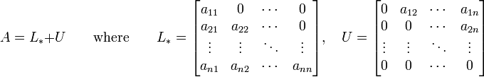
Then A can be decomposed into a lower triangular component L*, and a strictly upper triangular component U:
The system of linear equations may be rewritten as:

The Gauss–Seidel method is an iterative technique that solves the left hand side of this expression for x, using previous value for x on the right hand side. Analytically, this may be written as:

However, by taking advantage of the triangular form of L*, the elements of x(k+1) can be computed sequentially using forward substitution:
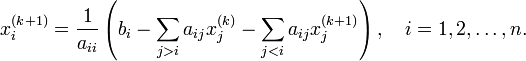
Note that the sum inside this computation of xi(k+1) requires each element in x(k) except xi(k) itself.
The procedure is generally continued until the changes made by an iteration are below some tolerance.
Discussion
The element-wise formula for the Gauss–Seidel method is extremely similar to that of the Jacobi method.
The computation of xi(k+1) uses only the elements of x(k+1) that have already been computed, and only the elements of x(k) that have yet to be advanced to iteration k+1. This means that, unlike the Jacobi method, only one storage vector is required as elements can be overwritten as they are computed, which can be advantageous for very large problems.
However, unlike the Jacobi method, the computations for each element cannot be done in parallel. Furthermore, the values at each iteration are dependent on the order of the original equations.
LU Decomposition
In linear algebra, the LU decomposition is a matrix decomposition which writes a matrix as the product of a lower triangular matrixpermutation matrix as well. This decomposition is used in numerical analysis to solve systems of linear equations or calculate the determinant and an upper triangular matrix. The product sometimes includes a permutation matrix as well. This decomposition is used in numerical analysis to solve systems of linear equations or calculate the determinante.
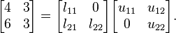
Let A be a square matrix. An LU decomposition is a decomposition of the form

where L and U are lower and upper triangular matrices (of the same size), respectively. This means that L has only zeros above the diagonal and U has only zeros below the diagonal. For a  matrix, this becomes:
matrix, this becomes:
The general equation to modify the terms
• - factor * pivot + position to change
So if Ax = b, then LUx = b, thus Ax = LUx = b
Example
One way of finding the LU decomposition of this simple matrix would be to simply solve the linear equations by inspection. You know that:
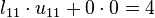
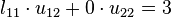

Such a system of equations is underdetermined. In this case any two non-zero elements of L and ULU matrices. For example, we can require the lower triangular matrix L matrices are parameters of the solution and can be set arbitrarily to any non-zero value. Therefore to find the unique LU decomposition, it is necessary to put some restriction on to be a unit one (i.e. set all the entries of its main diagonal to ones). Then the system of equations has the following solution: and
- l21 = 1.5
- u11 = 4
- u12 = 3
- u22 = − 1.5.
Substituting these values into the LU decomposition above:

Example
- l21 = 1.5
- u11 = 4
- u12 = 3
- u22 = − 1.5.
Jacobi's Method
This method had been consigned to history until the advent of parallel computing, but has now acquired a new lease of life. It uses a sequence of similarity transformations with plane rotation matrices, each one of which makes a larger than average off-diagonal element (and its transpose) zero. This unfortunately destroys previous zeros, but nevertheless reduces the sum of the off-diagonal elements, so that convergence to a diagonal matrix occurs.
The orthogonal matrix
![\begin{displaymath}P=\left[ \begin{array}{ccccccccccc}
1 & \cdots & \cdot & \cd...
...t]\begin{array}{c} \\ \\ s \\ \\ \\ \\ t \\ \\ \\ \end{array},
\end{displaymath}](http://www.maths.lancs.ac.uk/%7Egilbert/m306c/img259.gif)
where the non-standard elements are in rows and columns s and t, and real
![\begin{eqnarray*}[AP]_{ks} & = & a_{ks}\cos \phi
-a_{kt}\sin \phi \\ [0pt]
[AP]_...
...{kt}\cos \phi \\ [0pt]
[AP]_{kj} & = & a_{kj}, \quad j\not= s,t.
\end{eqnarray*}](http://www.maths.lancs.ac.uk/%7Egilbert/m306c/img261.gif)
Premultiplying by PT we find in particular that
and this is zero if
We could simply compute the sum of the squares of the off-diagonal elements, but we prefer a more roundabout approach.
Lemma 10.5.3 If B=PTAP, where P is orthogonal, then trace B= trace A and trace BTB= trace ATA.
Proof. The trace of a matrix is the sum of its eigenvalues, and A and B have the same eigenvalues, which proves the first part. Also BTB=(PTAP)TPTAP=PTATPPTAP=PT(ATA)P, and the first result now gives the second.
Now

In the case where
![$A=\left[ \begin{array}{ll}a_{ss} & a_{st}\\ a_{st} &
a_{tt}\end{array} \right]$](http://www.maths.lancs.ac.uk/%7Egilbert/m306c/img265.gif) , PTAP=B gives
, PTAP=B gives But each of these elements is just the same as in the

so the sum of the squares of the diagonal elements is increased by the transformation by an amount 2ast2. we now see that

where the sums are over all values of i,j which are not equal, that is over all off-diagonal elements.
If we choose ast so that  , that is, so that it is greater than average, we have
, that is, so that it is greater than average, we have 
and the sum of the off-diagonal elements converges to zero with convergence factor
Suppose the sequence of transformations is given by
with B0=A, and Pm chosen as above. Then Bm converges to a diagonal matrix whose elements are the eigenvalue sof A. When we have reached a sufficient degree of convergence, say for m=M, we have
say, and the eigenvectors of A are approximated by the columns of QM.
Special Sistems
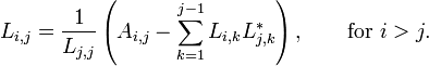
Cholesky Method
In linear algebra, the Cholesky decomposition or Cholesky triangle is a decomposition of a symmetric, positive-definite matrix into the product of a lower triangular matrix and its conjugate transpose. It was discovered by André-Louis Cholesky for real matrices and is an example of a square root of a matrix. When it is applicable, the Cholesky decomposition is roughly twice as efficient as the LU decomposition for solving systems of linear equations.
U=Lt
AX=b
LLtX=b

No hay comentarios:
Publicar un comentario